Molecular Dynamics Background

What is a Molecular Dynamics Simulation?¶

A molecular dynamics (MD) simulation is a computer experiment that tracks how atoms move over time. At every step, the computer looks at where the atoms are, calculates the forces between them, and nudges each atom forward by a tiny amount. That tiny amount is called the timestep, and it is usually about one femtosecond (10^-15 seconds). String millions of these steps together and you get a movie of atomic motion. The heart of any MD simulation is the potential. The potential assigns an energy to an atomic configuration, and the forces on the atoms are obtained from how that energy changes with their positions. Without a potential, there are no forces, and nothing moves.

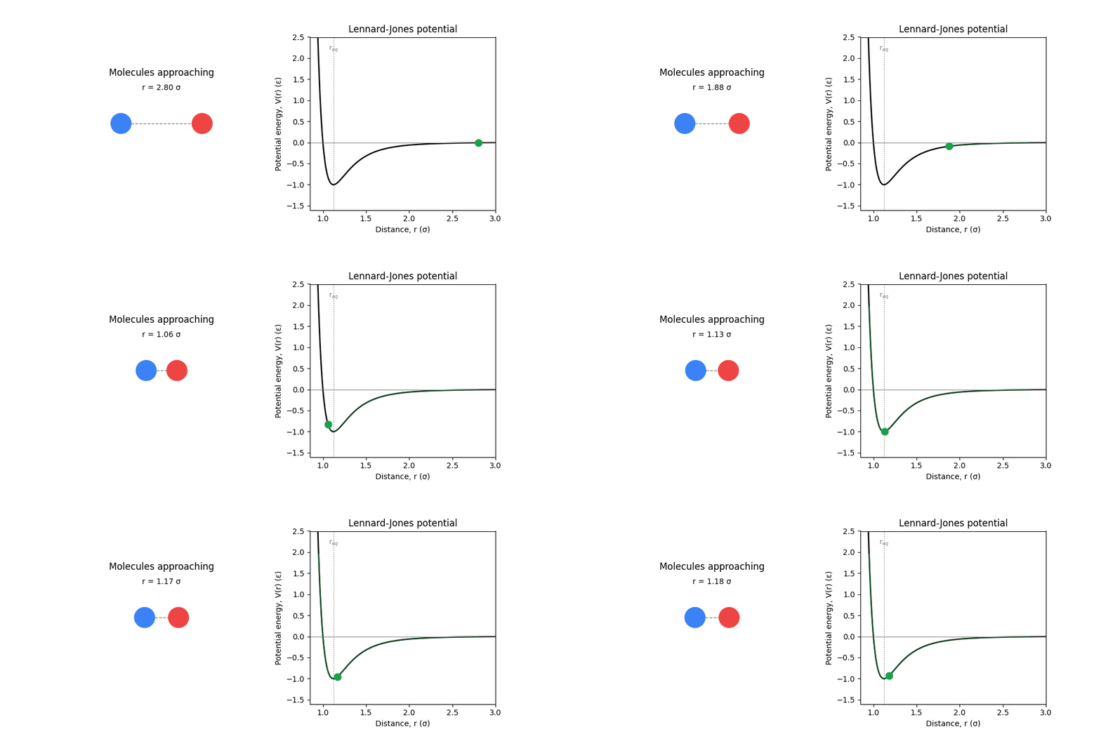
Lennard-Jones Potential Animation

There are two ways to build a potential:

Classical potentials are written down using physics. Someone studies the chemistry of a material, picks a functional form (like Lennard-Jones for noble gases or EAM for metals), and fits a few parameters. These are fast and interpretable, but each one is tailored to a specific system.

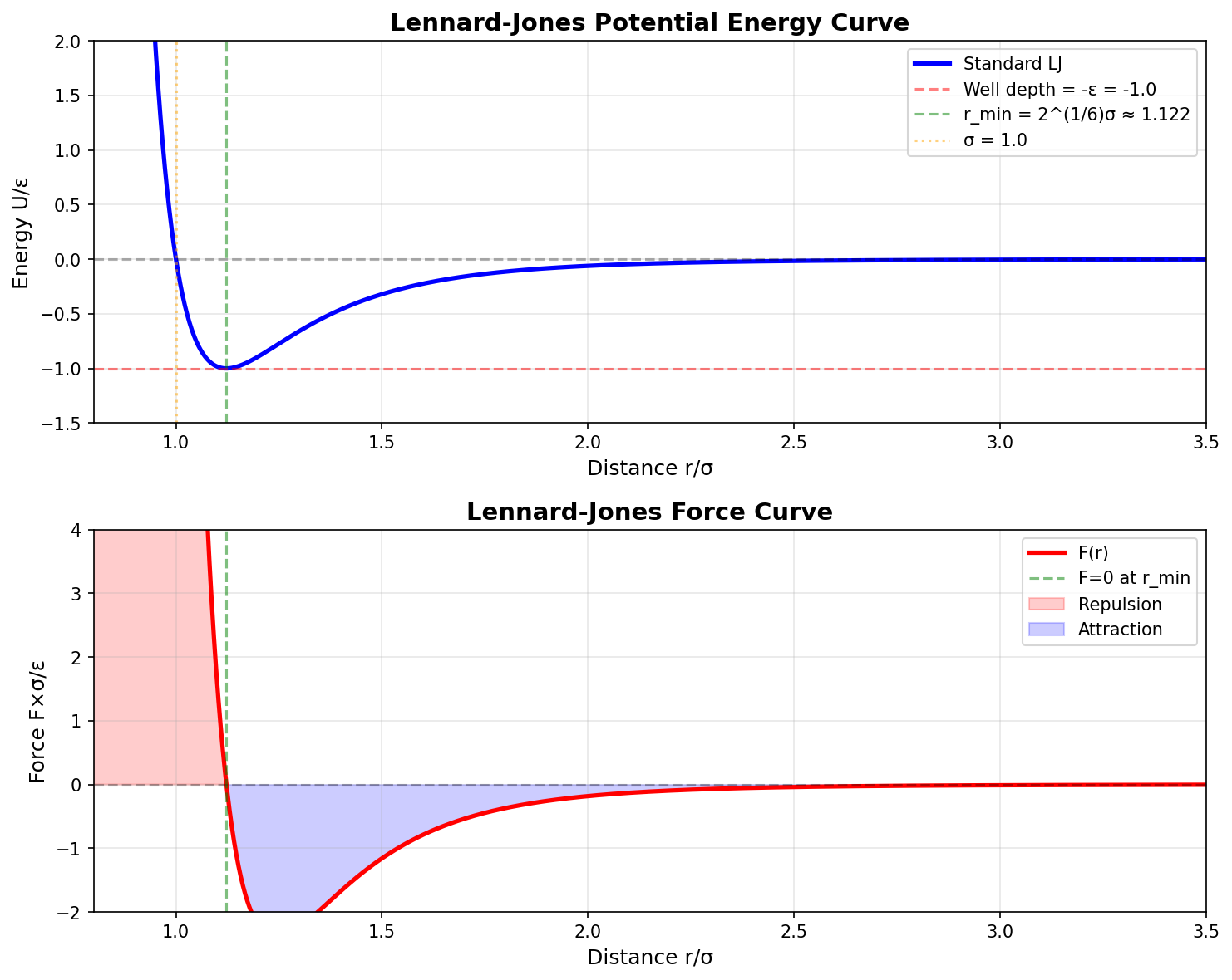
Image of Lennard-Jones Potential [1]

Machine learning (ML) potentials, like MACE (Message Passing Atomic Cluster Expansion) [2], take a different approach. Instead of writing down a physics-based formula, we train a neural network on a large dataset of accurate quantum mechanical calculations. The network learns the relationship between atomic arrangements and energies directly from the data. Once trained, it predicts energies and forces on new configurations quickly, often with accuracy close to the underlying quantum calculations.

Both approaches give the MD simulation the same thing: a way to calculate forces so atoms can be moved forward in time. The difference is in how that function is built. Classical potentials come from physical intuition. ML potentials come from data.

Why Cartesian Coordinates are used¶

When we set up an MD simulation, we have to pick a coordinate system to describe where each atom is. In principle, we could use internal coordinates (geometry defined based on bond lengths and angles) or polar coordinates, but almost every MD code uses plain Cartesian coordinates: each atom gets an (x, y, z) position and a velocity in each direction. There are two main reasons for this.

The equations of motion are simpler: In Cartesian coordinates, Newton’s equations can be written directly as separate x, y, and z component-wise updates for each atom. Internal coordinates couple the directions together, and the integrator has to untangle them at every step. That extra work is expensive, especially for large systems.

Bookkeeping scales cleanly:

A simulation box might contain thousands of molecules translating, rotating, and colliding. In Cartesian coordinates, every atom is described the same way regardless of what molecule it belongs to. Internal coordinates would require tracking which atom is bonded to which and updating those relationships as molecules move or react, which quickly becomes challenging.

Because these advantages are so strong for MD, the entire software ecosystem (LAMMPS [3], GROMACS [4], trajectory formats, analysis tools, visualizers) is built around Cartesian coordinates.

MACE Model Sizes¶

When you load a MACE-MP-0 model as “small”, “medium”, or “large”, the sizes do not refer to the training data. All three models are trained on the same Materials Project dataset (about 1.5 million atomic configurations covering 89 elements) and use the same underlying MACE architecture. What differs is the internal feature representation each atom carries through the network, which grows from about 3.8 million parameters in the small model, to 4.7 million in the medium, to 5.7 million in the large. A larger internal representation lets the model capture more subtle chemistry, at the cost of slower computation per timestep. In practice, the small model is useful for quick screening or very large systems, the large model is worth it when you need high accuracy on a small system, and the medium model is the recommended default for almost everything in between. For class-sized simulations on Anvil [5], a U.S. academic high-performance computing (HPC) cluster, the medium model is a reasonable starting point.

Stability and Optimization of MD Systems¶

All molecules have a stable form that corresponds to their minimum energy. Left alone, they naturally settle into this state. A geometry optimization uses a numerical algorithm to nudge the atoms toward that stable form before the simulation begins. The algorithm makes small adjustments to each atom’s position, checks whether the total potential energy went down, and repeats until the forces on every atom fall below a small threshold. A useful mental picture is a spring at its natural length. If we start the simulation with the spring already stretched or compressed, it will snap violently the moment we let go, and the dynamics will explode. Geometry optimization lets the spring relax first, so the system begins from a calm state rather than one primed to fly apart.

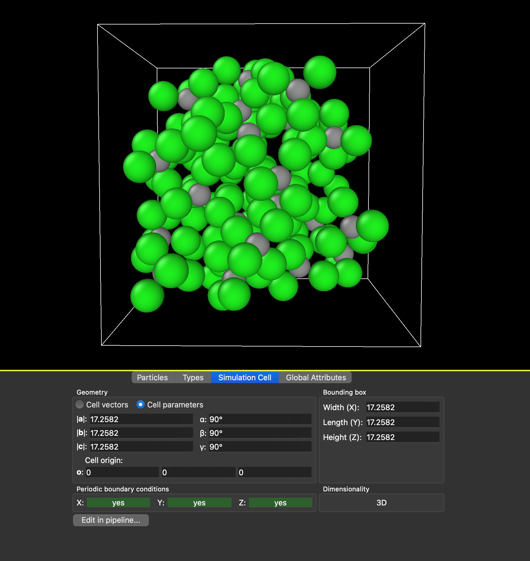
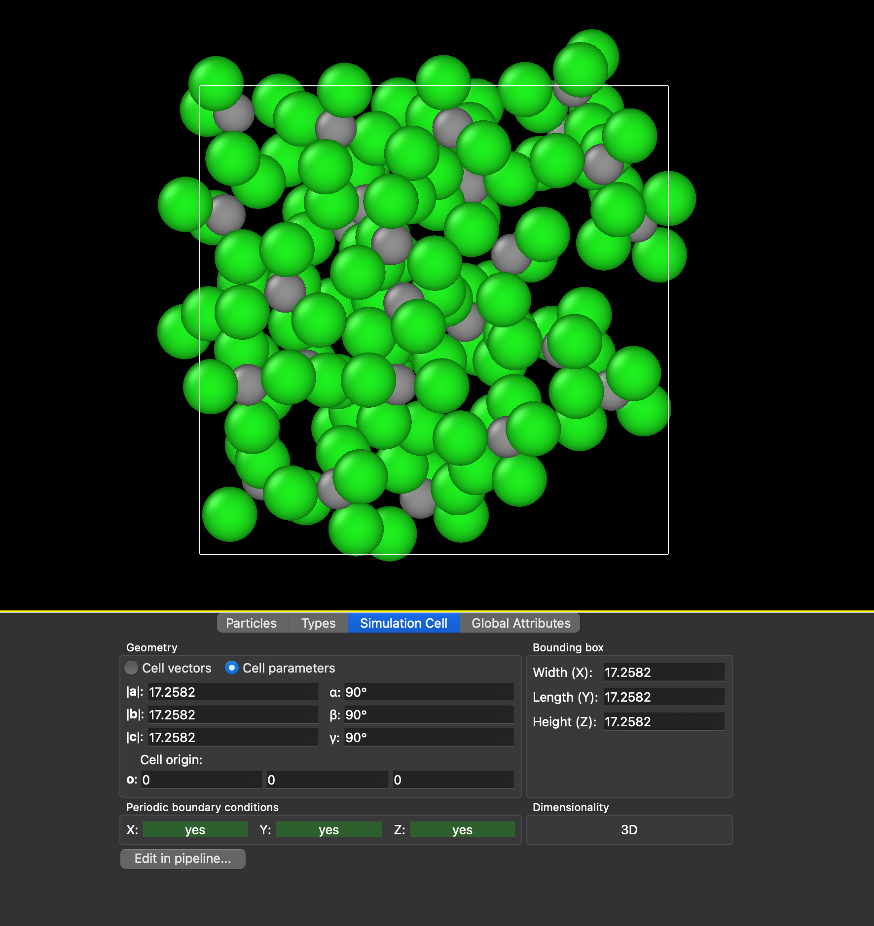
Reference State for Potential Energy Calculation and Ideal Gas Approximation¶

The potential energy that MACE (or any similar model) returns is not an absolute number with a universal zero. The zero point is set by the atomic reference energies used during training. The energy assigned to each isolated atom in the reference DFT calculations. This means the absolute value of the potential energy is not physically meaningful on its own. What is meaningful are differences in energy (reaction energies, binding energies, energy barriers), because the constant offset from the reference cancels out when you subtract.

For thermochemistry, we feed this potential energy along with the computed vibrational frequencies, the molecular geometry, symmetry number, spin, temperature, and pressure into a standard thermochemistry routine. This routine uses statistical mechanics under the ideal gas approximation: molecules do not interact with each other, they rotate as rigid bodies, they vibrate as harmonic oscillators, and they translate freely. Under these assumptions it computes the zero-point energy, the thermal vibrational, rotational, and translational contributions, and combines them into standard thermodynamic quantities like entropy, enthalpy, and Gibbs free energy.

Machine Learning Values and Obtaining Thermodynamic Properties¶

The machine learning model gives us one number for a given molecular geometry: the electronic energy E_elec. But a real molecule at room temperature is not sitting still. It vibrates, it rotates, and it translates through space. Each of these motions carries energy and contributes to the thermodynamic properties we actually care about, like enthalpy and Gibbs free energy. So how do we get from that one ML number to a full thermodynamic description? The answer comes from statistical mechanics, which connects the behavior of individual molecules to bulk thermodynamic quantities. Under the ideal gas approximation (molecules do not interact, they rotate as rigid bodies, and they vibrate like tiny springs), statistical mechanics gives provides well-defined expressions for each contribution. The inputs it needs are:

1. The electronic energy E_elec (from MACE)

2. The vibrational frequencies of the molecule (computed by slightly displacing each atom and re-evaluating the forces with MACE)

3. The molecular geometry, mass, and symmetry

4. The temperature and pressure

from these ingredients, standard formulas give the enthalpy H, which is the total energy content of the molecule plus a pressure-volume term:

Each term has a clear physical meaning. E_ZPE is the zero-point energy, the residual vibrational energy that molecules retain even at 0 K. The three thermal terms E_vib, E_rot, and E_trans are the additional energy the molecule holds because it is vibrating, rotating, and translating at temperature T. The PV term comes from the ideal gas law. The entropy S measures how many different microscopic states the molecule can occupy at a given temperature. More accessible states means higher entropy. Statistical mechanics gives separate contributions from translation, rotation, and vibration, which are added together.

Finally, the Gibbs free energy follows from its familiar thermodynamic definition:

The overall workflow is therefore: MACE provides the potential energy and the forces needed for vibrational frequencies, and statistical mechanics converts those microscopic quantities into the enthalpy, entropy, and free energy that engineers use every day.

Tutorials¶

Tutorial 1: Performing a molecular simulation using MACE-OFF, which will be used to calculate chemical properties of a molecule.

Tutorial 2: Performing multiple molecular simulations using MACE-OFF, which will be used to calculate the heat capacity of multiple molecules. Also some of the molecules will be constructed using RDKit.

Tutorial 3: Use a given database to calculate standard enthalpy of formation instead of performing molecular simulations.

Model Validation Metrics: Calculate standard enthalpy of formation using both molecular simulations as well as the database, and compare those values to the Database.

These Modules were made to instruct you on how to perform molecular simulations to calculate unknown or missing thermodynamic properties of new chemicals. These values will be used as inputs in phase 2 where you will be performing a life cycle assessment (LCA) of different chemicals.