Tutorial 2: Thermochemical Property Estimation (Heat Capacity for Gases)
In this tutorial you will learn how to compute the heat capacity of a gas using Machine Learning Potential (MACE-OFF) and the Atomic Simulation Environment (ASE)
Background Information:
The molar heat capacity at constant pressure, describes how the enthalpy of a substance changes with temperature at constant pressure. This code estimate this value using the idea that at constant pressure, the change in enthalpy with respect to the change in temperature is equal to the heat capacity.
From here we solve this derivative numerically instead of analytically, using a method called finite difference, which evaluates the derivative by finding the function values at temperatures that are close to the desired temperature and solving for the slope between the points.
Code Overview:
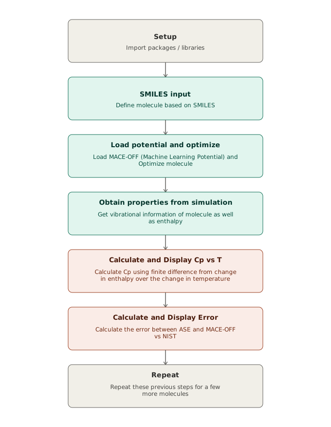
This code will define a molecule using SMILES and will create the geometry of the molecule. MACE-OFF will then optimize the geometry to ensure forces don’t explode initially. Then you will obtain some chemical properties of the molecules and use them to estimate the heat capacity at constant pressure. After that, the code will display this property and compare to NIST.
The libraries / packages listed in cell 2 will have a brief explanation of their function in the code, but for more information, please use the links below
| Library / Package | Link to Documentations |
|---|---|
| numpy | NumPy Documentation [8] |
| matplotlib.pyplot | Matplotlib.pyplot [19] |
| pandas | Pandas Documentation [9] |
| chem | rdkit.chem Documentation [10] |
| AllChem | Same link as above |
| Descriptors | Same link as above |
| rdMolDescriptors | Same Link as above |
| mace_off | MACE Calculator Documentation [11] |
| mace_off | MACE Descriptors Documentation [12] |
| atoms | Atoms Object Documentation [13] |
| units | Units Documentation [18] |
| LBFGS | Structure Optimization Documentation [15] |
| Vibrations | Vibrational Modes Documentation [16] |
| IdealGasThermo | Ideal-gas limit Documentation [17] |
Click the button below to open this code in Google Colab

Outputs Should Appear Like This:
# Cell 1: Import Required Packages

!pip install ASE
!pip install mace-torch
!pip install rdkit
Expected output
Collecting ASE
  Downloading ase-3.29.0-py3-none-any.whl.metadata (4.4 kB)
Requirement already satisfied: numpy>=1.21.6 in /usr/local/lib/python3.12/dist-packages (from ASE) (2.0.2)
Requirement already satisfied: scipy>=1.8.1 in /usr/local/lib/python3.12/dist-packages (from ASE) (1.16.3)
Requirement already satisfied: matplotlib>=3.5.2 in /usr/local/lib/python3.12/dist-packages (from ASE) (3.10.0)
Requirement already satisfied: typing_extensions>=4.13.1 in /usr/local/lib/python3.12/dist-packages (from ASE) (4.15.0)
Requirement already satisfied: contourpy>=1.0.1 in /usr/local/lib/python3.12/dist-packages (from matplotlib>=3.5.2->ASE) (1.3.3)
Requirement already satisfied: cycler>=0.10 in /usr/local/lib/python3.12/dist-packages (from matplotlib>=3.5.2->ASE) (0.12.1)
Requirement already satisfied: fonttools>=4.22.0 in /usr/local/lib/python3.12/dist-packages (from matplotlib>=3.5.2->ASE) (4.63.0)
Requirement already satisfied: kiwisolver>=1.3.1 in /usr/local/lib/python3.12/dist-packages (from matplotlib>=3.5.2->ASE) (1.5.0)
Requirement already satisfied: packaging>=20.0 in /usr/local/lib/python3.12/dist-packages (from matplotlib>=3.5.2->ASE) (26.2)
Requirement already satisfied: pillow>=8 in /usr/local/lib/python3.12/dist-packages (from matplotlib>=3.5.2->ASE) (11.3.0)
Requirement already satisfied: pyparsing>=2.3.1 in /usr/local/lib/python3.12/dist-packages (from matplotlib>=3.5.2->ASE) (3.3.2)
Requirement already satisfied: python-dateutil>=2.7 in /usr/local/lib/python3.12/dist-packages (from matplotlib>=3.5.2->ASE) (2.9.0.post0)
Requirement already satisfied: six>=1.5 in /usr/local/lib/python3.12/dist-packages (from python-dateutil>=2.7->matplotlib>=3.5.2->ASE) (1.17.0)
Downloading ase-3.29.0-py3-none-any.whl (3.0 MB)
   ━━━━━━━━━━━━━━━━━━━━━━━━━━━━━━━━━━━━━━━━ 3.0/3.0 MB 32.2 MB/s eta 0:00:00
Installing collected packages: ASE
Successfully installed ASE-3.29.0
Collecting mace-torch
  Downloading mace_torch-0.3.16-py3-none-any.whl.metadata (27 kB)
Requirement already satisfied: torch>=1.12 in /usr/local/lib/python3.12/dist-packages (from mace-torch) (2.11.0+cpu)
Collecting e3nn==0.4.4 (from mace-torch)
  Downloading e3nn-0.4.4-py3-none-any.whl.metadata (5.1 kB)
Requirement already satisfied: numpy in /usr/local/lib/python3.12/dist-packages (from mace-torch) (2.0.2)
Requirement already satisfied: opt_einsum in /usr/local/lib/python3.12/dist-packages (from mace-torch) (3.4.0)
Requirement already satisfied: ase in /usr/local/lib/python3.12/dist-packages (from mace-torch) (3.29.0)
Collecting torch-ema (from mace-torch)
  Downloading torch_ema-0.3-py3-none-any.whl.metadata (415 bytes)
Requirement already satisfied: prettytable in /usr/local/lib/python3.12/dist-packages (from mace-torch) (3.17.0)
Collecting matscipy (from mace-torch)
  Downloading matscipy-1.2.0-cp312-cp312-manylinux_2_24_x86_64.manylinux_2_28_x86_64.whl.metadata (37 kB)
Requirement already satisfied: h5py in /usr/local/lib/python3.12/dist-packages (from mace-torch) (3.16.0)
Collecting torchmetrics (from mace-torch)
  Downloading torchmetrics-1.9.0-py3-none-any.whl.metadata (23 kB)
Collecting python-hostlist (from mace-torch)
  Downloading python_hostlist-2.3.0.tar.gz (37 kB)
  Preparing metadata (setup.py) ... done
Collecting configargparse (from mace-torch)
  Downloading configargparse-1.7.5-py3-none-any.whl.metadata (23 kB)
Requirement already satisfied: GitPython in /usr/local/lib/python3.12/dist-packages (from mace-torch) (3.1.50)
Requirement already satisfied: pyYAML in /usr/local/lib/python3.12/dist-packages (from mace-torch) (6.0.3)
Requirement already satisfied: tqdm in /usr/local/lib/python3.12/dist-packages (from mace-torch) (4.67.3)
Collecting lmdb (from mace-torch)
  Downloading lmdb-2.2.1-cp312-cp312-manylinux2014_x86_64.manylinux_2_17_x86_64.manylinux_2_28_x86_64.whl.metadata (1.2 kB)
Requirement already satisfied: orjson in /usr/local/lib/python3.12/dist-packages (from mace-torch) (3.11.9)
Requirement already satisfied: matplotlib in /usr/local/lib/python3.12/dist-packages (from mace-torch) (3.10.0)
Requirement already satisfied: pandas in /usr/local/lib/python3.12/dist-packages (from mace-torch) (2.2.2)
Requirement already satisfied: sympy in /usr/local/lib/python3.12/dist-packages (from e3nn==0.4.4->mace-torch) (1.14.0)
Requirement already satisfied: scipy in /usr/local/lib/python3.12/dist-packages (from e3nn==0.4.4->mace-torch) (1.16.3)
Collecting opt-einsum-fx>=0.1.4 (from e3nn==0.4.4->mace-torch)
  Downloading opt_einsum_fx-0.1.4-py3-none-any.whl.metadata (3.3 kB)
Requirement already satisfied: filelock in /usr/local/lib/python3.12/dist-packages (from torch>=1.12->mace-torch) (3.29.3)
Requirement already satisfied: typing-extensions>=4.10.0 in /usr/local/lib/python3.12/dist-packages (from torch>=1.12->mace-torch) (4.15.0)
Requirement already satisfied: setuptools<82 in /usr/local/lib/python3.12/dist-packages (from torch>=1.12->mace-torch) (75.2.0)
Requirement already satisfied: networkx>=2.5.1 in /usr/local/lib/python3.12/dist-packages (from torch>=1.12->mace-torch) (3.6.1)
Requirement already satisfied: jinja2 in /usr/local/lib/python3.12/dist-packages (from torch>=1.12->mace-torch) (3.1.6)
Requirement already satisfied: fsspec>=0.8.5 in /usr/local/lib/python3.12/dist-packages (from torch>=1.12->mace-torch) (2025.3.0)
Requirement already satisfied: contourpy>=1.0.1 in /usr/local/lib/python3.12/dist-packages (from matplotlib->mace-torch) (1.3.3)
Requirement already satisfied: cycler>=0.10 in /usr/local/lib/python3.12/dist-packages (from matplotlib->mace-torch) (0.12.1)
Requirement already satisfied: fonttools>=4.22.0 in /usr/local/lib/python3.12/dist-packages (from matplotlib->mace-torch) (4.63.0)
Requirement already satisfied: kiwisolver>=1.3.1 in /usr/local/lib/python3.12/dist-packages (from matplotlib->mace-torch) (1.5.0)
Requirement already satisfied: packaging>=20.0 in /usr/local/lib/python3.12/dist-packages (from matplotlib->mace-torch) (26.2)
Requirement already satisfied: pillow>=8 in /usr/local/lib/python3.12/dist-packages (from matplotlib->mace-torch) (11.3.0)
Requirement already satisfied: pyparsing>=2.3.1 in /usr/local/lib/python3.12/dist-packages (from matplotlib->mace-torch) (3.3.2)
Requirement already satisfied: python-dateutil>=2.7 in /usr/local/lib/python3.12/dist-packages (from matplotlib->mace-torch) (2.9.0.post0)
Requirement already satisfied: gitdb<5,>=4.0.1 in /usr/local/lib/python3.12/dist-packages (from GitPython->mace-torch) (4.0.12)
Requirement already satisfied: pytz>=2020.1 in /usr/local/lib/python3.12/dist-packages (from pandas->mace-torch) (2025.2)
Requirement already satisfied: tzdata>=2022.7 in /usr/local/lib/python3.12/dist-packages (from pandas->mace-torch) (2026.2)
Requirement already satisfied: wcwidth in /usr/local/lib/python3.12/dist-packages (from prettytable->mace-torch) (0.8.1)
Collecting lightning-utilities>=0.15.3 (from torchmetrics->mace-torch)
  Downloading lightning_utilities-0.15.3-py3-none-any.whl.metadata (5.5 kB)
Requirement already satisfied: smmap<6,>=3.0.1 in /usr/local/lib/python3.12/dist-packages (from gitdb<5,>=4.0.1->GitPython->mace-torch) (5.0.3)
Requirement already satisfied: six>=1.5 in /usr/local/lib/python3.12/dist-packages (from python-dateutil>=2.7->matplotlib->mace-torch) (1.17.0)
Requirement already satisfied: mpmath<1.4,>=1.1.0 in /usr/local/lib/python3.12/dist-packages (from sympy->e3nn==0.4.4->mace-torch) (1.3.0)
Requirement already satisfied: MarkupSafe>=2.0 in /usr/local/lib/python3.12/dist-packages (from jinja2->torch>=1.12->mace-torch) (3.0.3)
Downloading mace_torch-0.3.16-py3-none-any.whl (316 kB)
   ━━━━━━━━━━━━━━━━━━━━━━━━━━━━━━━━━━━━━━━━ 316.0/316.0 kB 16.2 MB/s eta 0:00:00
Downloading e3nn-0.4.4-py3-none-any.whl (387 kB)
   ━━━━━━━━━━━━━━━━━━━━━━━━━━━━━━━━━━━━━━━━ 387.7/387.7 kB 18.7 MB/s eta 0:00:00
Downloading configargparse-1.7.5-py3-none-any.whl (27 kB)
Downloading lmdb-2.2.1-cp312-cp312-manylinux2014_x86_64.manylinux_2_17_x86_64.manylinux_2_28_x86_64.whl (338 kB)
   ━━━━━━━━━━━━━━━━━━━━━━━━━━━━━━━━━━━━━━━━ 338.3/338.3 kB 16.8 MB/s eta 0:00:00
Downloading matscipy-1.2.0-cp312-cp312-manylinux_2_24_x86_64.manylinux_2_28_x86_64.whl (453 kB)
   ━━━━━━━━━━━━━━━━━━━━━━━━━━━━━━━━━━━━━━━━ 453.1/453.1 kB 21.7 MB/s eta 0:00:00
Downloading torch_ema-0.3-py3-none-any.whl (5.5 kB)
Downloading torchmetrics-1.9.0-py3-none-any.whl (983 kB)
   ━━━━━━━━━━━━━━━━━━━━━━━━━━━━━━━━━━━━━━━━ 983.4/983.4 kB 38.0 MB/s eta 0:00:00
Downloading lightning_utilities-0.15.3-py3-none-any.whl (31 kB)
Downloading opt_einsum_fx-0.1.4-py3-none-any.whl (13 kB)
Building wheels for collected packages: python-hostlist
  Building wheel for python-hostlist (setup.py) ... done
  Created wheel for python-hostlist: filename=python_hostlist-2.3.0-py3-none-any.whl size=39449 sha256=ed8cadfb780777460ce616bd9eaf80c88fce107d48531bcfd05b94673e02daaf
  Stored in directory: /root/.cache/pip/wheels/02/e4/34/75fc0cd5b7889d8cc4ce6fb2f74c9fd17b3c6138cb03832481
Successfully built python-hostlist
Installing collected packages: python-hostlist, lmdb, lightning-utilities, configargparse, torchmetrics, torch-ema, opt-einsum-fx, matscipy, e3nn, mace-torch
Successfully installed configargparse-1.7.5 e3nn-0.4.4 lightning-utilities-0.15.3 lmdb-2.2.1 mace-torch-0.3.16 matscipy-1.2.0 opt-einsum-fx-0.1.4 python-hostlist-2.3.0 torch-ema-0.3 torchmetrics-1.9.0
Collecting rdkit
  Downloading rdkit-2026.3.3-cp312-cp312-manylinux_2_28_x86_64.whl.metadata (3.8 kB)
Requirement already satisfied: numpy in /usr/local/lib/python3.12/dist-packages (from rdkit) (2.0.2)
Requirement already satisfied: Pillow in /usr/local/lib/python3.12/dist-packages (from rdkit) (11.3.0)
Downloading rdkit-2026.3.3-cp312-cp312-manylinux_2_28_x86_64.whl (37.2 MB)
   ━━━━━━━━━━━━━━━━━━━━━━━━━━━━━━━━━━━━━━━━ 37.2/37.2 MB 26.3 MB/s eta 0:00:00
Installing collected packages: rdkit
Successfully installed rdkit-2026.3.3
Cell 1 Purpose: Install packages for ASE, MACE-OFF, and RDKit.
# Cell 2: Import Required Libraries

# Tools for plotting charts
import numpy as np                                # Computational library
import matplotlib.pyplot as plt                   # Plot graphs
import pandas as pd                               # Excel of python

# RDKit is for SMILES to construct a molecule
from rdkit import Chem                            # Used to build molecules (basic package)
from rdkit.Chem import AllChem, Descriptors       # Used to build molecules (advanced package)
from rdkit.Chem import rdMolDescriptors           # Used to obtain information of molecules

# MACE-OFF is the machine learning potential trained on organic molecules
from mace.calculators import mace_off             # MACE-OFF (Machine Learning Potential)

# ASE (Atomic Simulation Environment) computes information recieved from the machine learning potential
from ase import Atoms, units                      # Represents a molecule object with information and conversion for units
from ase.optimize import LBFGS                    # Optimization / energy minimization
from ase.vibrations import Vibrations             # Used to calculate vibrational modes of the Atom object
from ase.thermochemistry import IdealGasThermo    # Allows you to calculate entropy, enthalpy, and gibbs free energy
Expected output
/usr/local/lib/python3.12/dist-packages/e3nn/o3/_wigner.py:10: UserWarning: Environment variable TORCH_FORCE_NO_WEIGHTS_ONLY_LOAD detected, since the`weights_only` argument was not explicitly passed to `torch.load`, forcing weights_only=False.
  _Jd, _W3j_flat, _W3j_indices = torch.load(os.path.join(os.path.dirname(__file__), 'constants.pt'))
cuequivariance or cuequivariance_torch is not available. Cuequivariance acceleration will be disabled.
Cell 2 Purpose: Import required libraries to run codes in subsequent cells.
# Cell 3: Define Molecule using Simplified Molecular Input Line Entry System (SMILES) to construct it

SMILES = "O=C=O"          # Carbon Dioxide


# Other examples to try:
# SMILES = "CC(=O)O"    # Acetic acid
# SMILES = "c1ccccc1"   # Benzene
# SMILES = "CCCC"       # Butane

TEMPERATURE_K  = 298.15   # Temperature in [K] (temperature focused on in the chart below)
MODEL_SIZE     = "medium"  # 'small' (fast) | 'medium' | 'large' (A greater size generally correlates to higher accuracy with the cost of computational time)
DEVICE         = "cpu"    # 'cpu' or 'cuda' (Determines what the code will be running on, a cpu or cuda core (gpu))
FMAX           = 0.01     # eV/Å optimisation threshold use between 0.01 and 0.05 depending on how long the code runs for (higher threshold runs faster)
Cell 3 Purpose: Defines carbon dioxide molecule using SMILES and some input parameters for using MACE-OFF in subsequent cells
Carbon Dioxide
SMILES: O=C=O
Chemical Formula: CO2
Click the power icon and then run the cell below to view an interactive model of a Carbon Dioxide Molecule
import micropip
await micropip.install("py3Dmol")

from pyodide.http import pyfetch
import py3Dmol


response = await pyfetch("https://raw.githubusercontent.com/cacherowan/CACHE-Rowan/main/Reference_Files/Molecules_To_View/Carbon_Dioxide(CO_2).xyz")
xyz = await response.string()

view = py3Dmol.view(width=800, height=400)
view.addModel(xyz, "xyz")
view.setStyle({"stick": {}, "sphere": {"scale": 0.3}})
view.zoomTo()
view.zoom(2)
view.show()
# Cell 4: Defines Fucntion that takes a SMILES and returns if it is valid. Then it prints some information about the molecule
SUPPORTED_ELEMENTS = {"C", "H", "N", "O", "F", "Cl", "Br", "S", "P"} # Elements that MACE-OFF is trained on (it should get accurate results with molecules made of these elements)
def validate_smiles(smiles):
"""Validate SMILES and check element compatibility with MACE-OFF."""
mol = Chem.MolFromSmiles(smiles)
if mol is None:
raise ValueError(f"Invalid SMILES string: '{smiles}'")
mol = Chem.AddHs(mol) # add explicit hydrogens
elements = {atom.GetSymbol() for atom in mol.GetAtoms()}
unsupported = elements - SUPPORTED_ELEMENTS
if unsupported:
raise ValueError(
f"Unsupported elements for MACE-OFF: {unsupported}\n"
f"MACE-OFF supports: {SUPPORTED_ELEMENTS}"
)
formula = rdMolDescriptors.CalcMolFormula(mol)
mw = Descriptors.MolWt(mol)
print(f" SMILES : {smiles}")
print(f" Formula : {formula}")
print(f" Mol. wt : {mw:.2f} g/mol")
print(f" Elements : {elements}")
print(f" MACE-OFF compatible: ✓")
return mol, formula, mw
print("Validating molecule...")
rdkit_mol, formula, mol_weight = validate_smiles(SMILES)Expected output
Validating molecule...
  SMILES   : O=C=O
  Formula  : CO2
  Mol. wt  : 44.01 g/mol
  Elements : {'C', 'O'}
  MACE-OFF compatible: ✓
Cell 4 Purpose: Validates SMILES and outputs some property information.
# Cell 5: Defines Function to Create Atom layout to be optimized later by MACE-OFF

def smiles_to_ase(smiles):
    """Convert SMILES - RDKit 3D - ASE Atoms object."""
    mol = Chem.MolFromSmiles(smiles)
    mol = Chem.AddHs(mol)

    # Embed 3D coordinates
    params = AllChem.ETKDGv3()
    params.randomSeed = 42
    result = AllChem.EmbedMolecule(mol, params)
    if result != 0:
        raise RuntimeError("RDKit failed to generate 3D coordinates.")

    # Pre-optimise with MMFF94 (gives MACE-OFF a better starting point)
    AllChem.MMFFOptimizeMolecule(mol, maxIters=2000)

    # Extract positions and elements
    conf = mol.GetConformer()
    positions = conf.GetPositions()   # Angstrom
    symbols   = [atom.GetSymbol() for atom in mol.GetAtoms()]

    return Atoms(symbols=symbols, positions=positions)

atoms = smiles_to_ase(SMILES)
print(f"3D structure generated: {len(atoms)} atoms")
print(f"Symbols: {atoms.get_chemical_symbols()}")
Expected output
3D structure generated: 3 atoms
Symbols: ['O', 'C', 'O']
Cell 5 Purpose: After validation of SMILES, this cell takes the SMILES and constructs the molecule using RDKit.
# Cell 6: Loads MACE-OFF and moves atoms (slightly) around until the forces on them fall under the input threshold below (this is done to avoid huge forces initially ruining the simulation)

print(f"Loading MACE-OFF ({MODEL_SIZE}) on {DEVICE}...")
calc = mace_off(model=MODEL_SIZE, device=DEVICE)
print("Calculator ready.\n")

# Attach calculator and optimise
atoms.calc = calc
print("Optimising geometry with MACE-OFF...")
opt = LBFGS(atoms, logfile=None)
opt.run(fmax=FMAX)

E0 = atoms.get_potential_energy()   # eV
print(f"Optimisation complete.")
print(f"  Energy        : {E0:.6f} eV = {E0 * 96.485:.6f} kJ")
print(f"  Max force     : {np.max(np.linalg.norm(atoms.get_forces(), axis=1)):.4f} eV/Å")
Expected output
Loading MACE-OFF (medium) on cpu...
Downloading MACE model from 'https://raw.githubusercontent.com/ACEsuit/mace-off/main/mace_off23/MACE-OFF23_medium.model'
The model is distributed under the Academic Software License (ASL) license, see https://github.com/gabor1/ASL
 To use the model you accept the terms of the license.
ASL is based on the Gnu Public License, but does not permit commercial use
Downloading: 100.0% (17.5 MB / 17.5 MB)
Cached MACE model to /root/.cache/mace/MACE-OFF23_medium.model
Using MACE-OFF23 MODEL for MACECalculator with /root/.cache/mace/MACE-OFF23_medium.model
Using float64 for MACECalculator, which is slower but more accurate. Recommended for geometry optimization.
/usr/local/lib/python3.12/dist-packages/mace/calculators/mace.py:226: UserWarning: Environment variable TORCH_FORCE_NO_WEIGHTS_ONLY_LOAD detected, since the`weights_only` argument was not explicitly passed to `torch.load`, forcing weights_only=False.
  torch.load(f=model_path, map_location=device)
Calculator ready.

Optimising geometry with MACE-OFF...
Optimisation complete.
  Energy        : -5135.151897 eV = -495465.130773 kJ
  Max force     : 0.0048 eV/Å
Cell 6 Purpose: Load MACE-OFF and optimize molecule.
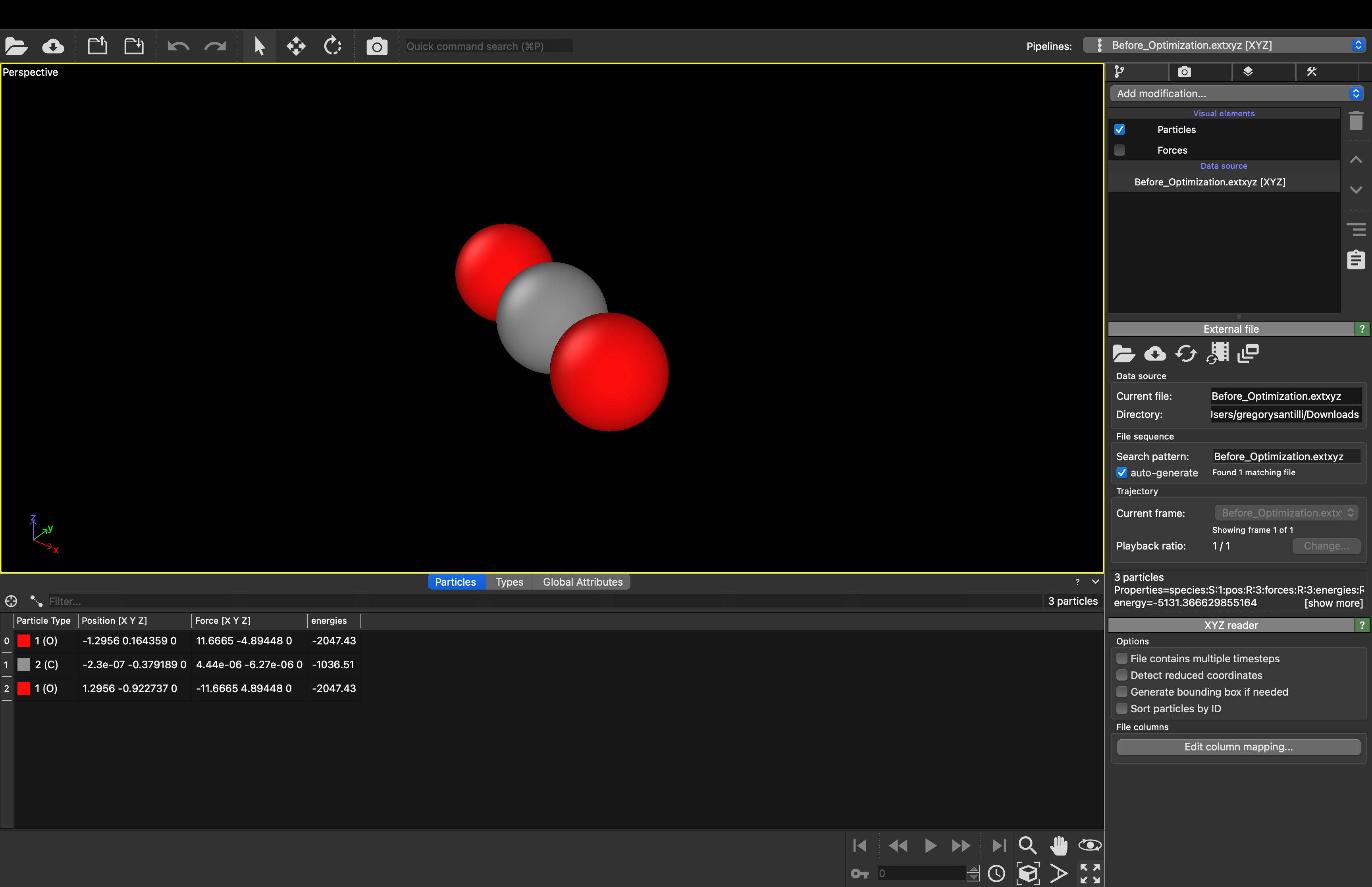 | 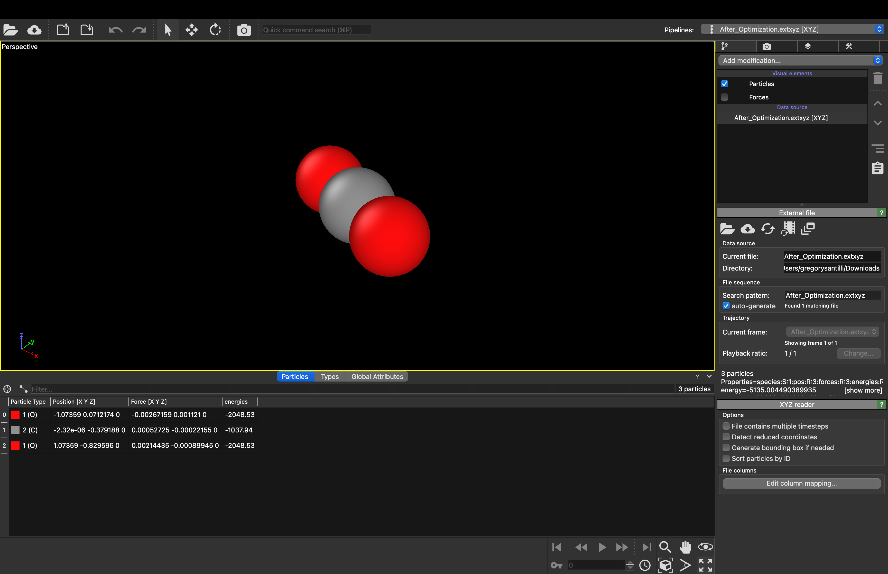 |
|---|---|
| Image of carbon dioxide molecule before optimization (No visible difference with other image) | Image of carbon dioxide molecule optimized (No visible difference with other image) |
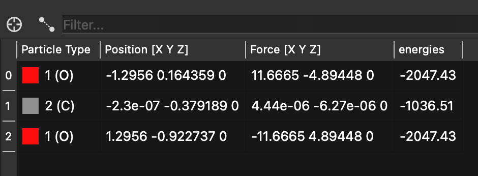 | 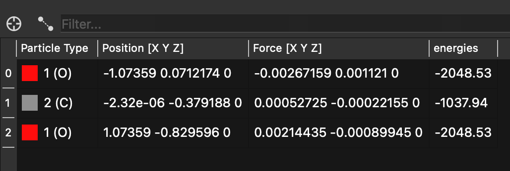 |
| Notice the forces are much higher in the x, y, and z directions for each atom | Notice how the forces are much lower in the x, y, and z directions for each atom (optimized or minimized) |
# Cell 7: Finds the potential energy of the molecule including vibrational energy (also filters out imaginary frequencies)

from pathlib import Path
import shutil

# Clear stale cache
shutil.rmtree("vib_cache", ignore_errors=True)

vib_dir = Path("vib_cache")
vib_dir.mkdir(exist_ok=True)

print(f"Running vibrational analysis ({3 * len(atoms)} force evaluations)...")
vib = Vibrations(atoms, name=str(vib_dir / "vib"), delta=0.01)
vib.run()

# Get all energies
vib_energies = vib.get_energies()

# Filter out imaginary and near-zero frequencies
real_vib_energies = vib_energies[vib_energies.real > 0.01]

# Check for too many imaginary modes
n_imaginary = np.sum(vib_energies.real < 0)
if n_imaginary > 2:
    print(f"⚠️  Warning: {n_imaginary} imaginary frequencies detected.")
    print("    Consider tightening FMAX for more reliable results.")
else:
    print(f"✓  {n_imaginary} imaginary mode(s) filtered — looks clean.")

print(f"\nTotal modes      : {len(vib_energies)}")
print(f"Imaginary/zero   : {len(vib_energies) - len(real_vib_energies)}")
print(f"Real modes kept  : {len(real_vib_energies)}")

# Print frequencies manually in cm⁻¹
print("\nVibrational frequencies (real modes):")
freqs_cm = real_vib_energies.real * 8065.54   # eV → cm⁻¹
for i, f in enumerate(freqs_cm):
    print(f"  Mode {i+1:>3d}: {f:>10.2f} cm⁻¹")
Expected output
Running vibrational analysis (9 force evaluations)...
✓  0 imaginary mode(s) filtered — looks clean.

Total modes      : 9
Imaginary/zero   : 5
Real modes kept  : 4

Vibrational frequencies (real modes):
  Mode   1:     673.48 cm⁻¹
  Mode   2:     673.87 cm⁻¹
  Mode   3:    1384.89 cm⁻¹
  Mode   4:    2395.61 cm⁻¹
Cell 7 Purpose: Find the total energy of the molecule including vibrational energy. This cell also filters out imaginary frequencies.
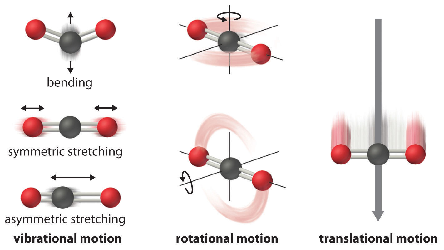
Possible Molecular Motion [20]
# Cell 8: Determines characteristics of the molecule to accurately compute chemical properties


#**** It is correct for this tutorial, but if you change molecules / atoms, make sure to change the geometry, symmetry, and spin below in this cell****


thermo = IdealGasThermo(
    vib_energies=real_vib_energies,
    potentialenergy=E0,
    atoms=atoms,
    geometry='linear',  # Change to match molecule (Linear or nonlinear)
    symmetrynumber=2,   # Change to match molecule (how many times you can turn the molecule and have symmetry)
    spin=0,             # Change to match molecule (0.5 times number of unpaired electrons)
)

# Uses the Constant Pressure Enthalpy Equation

# Cp via finite-difference dH/dT
def get_Cp_JmolK(T, dT=1.0):
    H_p = thermo.get_enthalpy(T + dT, verbose=False)
    H_m = thermo.get_enthalpy(T - dT, verbose=False)
    return (H_p - H_m) / (2 * dT) * 96485.3   # eV/K to J/(mol·K)

Cp_ref = get_Cp_JmolK(TEMPERATURE_K)

print(f"\n{'='*45}")
print(f"  GAS HEAT CAPACITY — {formula}")
print(f"  T = {TEMPERATURE_K} K")
print(f"{'='*45}")
print(f"  Cₚ = {Cp_ref:>8.2f}  J/(mol·K)")
print(f"{'='*45}")
Expected output
=============================================
  GAS HEAT CAPACITY — CO2
  T = 298.15 K
=============================================
  Cₚ =    36.94  J/(mol·K)
=============================================
Cell 8 Purpose: Uses IdealGasThermo class to the enthalpy of the molecule. Then you use finite difference to estimate the heat capacity of a molecule at a specific temperature.
# Cell 9: Cp vs T curve

# Rigid-Rotor Harmonic-Oscillator (Tracks atomic roational energy, not stretching at all, and treats bonds like springs)

# temps is the x-axis range of the graph and Cp_vals calls the function previously used to compute the y value or Cp for all x values, using a step up and step down to compute
temps = np.linspace(200, 1000, 80)
Cp_vals = [get_Cp_JmolK(T) for T in temps]

fig, ax = plt.subplots(figsize=(8, 4))
ax.plot(temps, Cp_vals, color="steelblue", lw=2.5)
ax.axvline(TEMPERATURE_K, color="gray", ls="--", alpha=0.7,
           label=f"T = {TEMPERATURE_K} K  →  Cₚ = {Cp_ref:.1f} J/(mol·K)")
ax.scatter([TEMPERATURE_K], [Cp_ref], color="tomato", zorder=5, s=60)
ax.set_xlabel("Temperature (K)", fontsize=12)
ax.set_ylabel("Cₚ  [J / (mol·K)]", fontsize=12)
ax.set_title(f"Gas-phase Cₚ(T) — {formula}  (MACE-OFF {MODEL_SIZE}, RRHO)", fontsize=12)
ax.legend(fontsize=10)
ax.grid(True, alpha=0.25)
plt.tight_layout()
plt.show()
Expected output
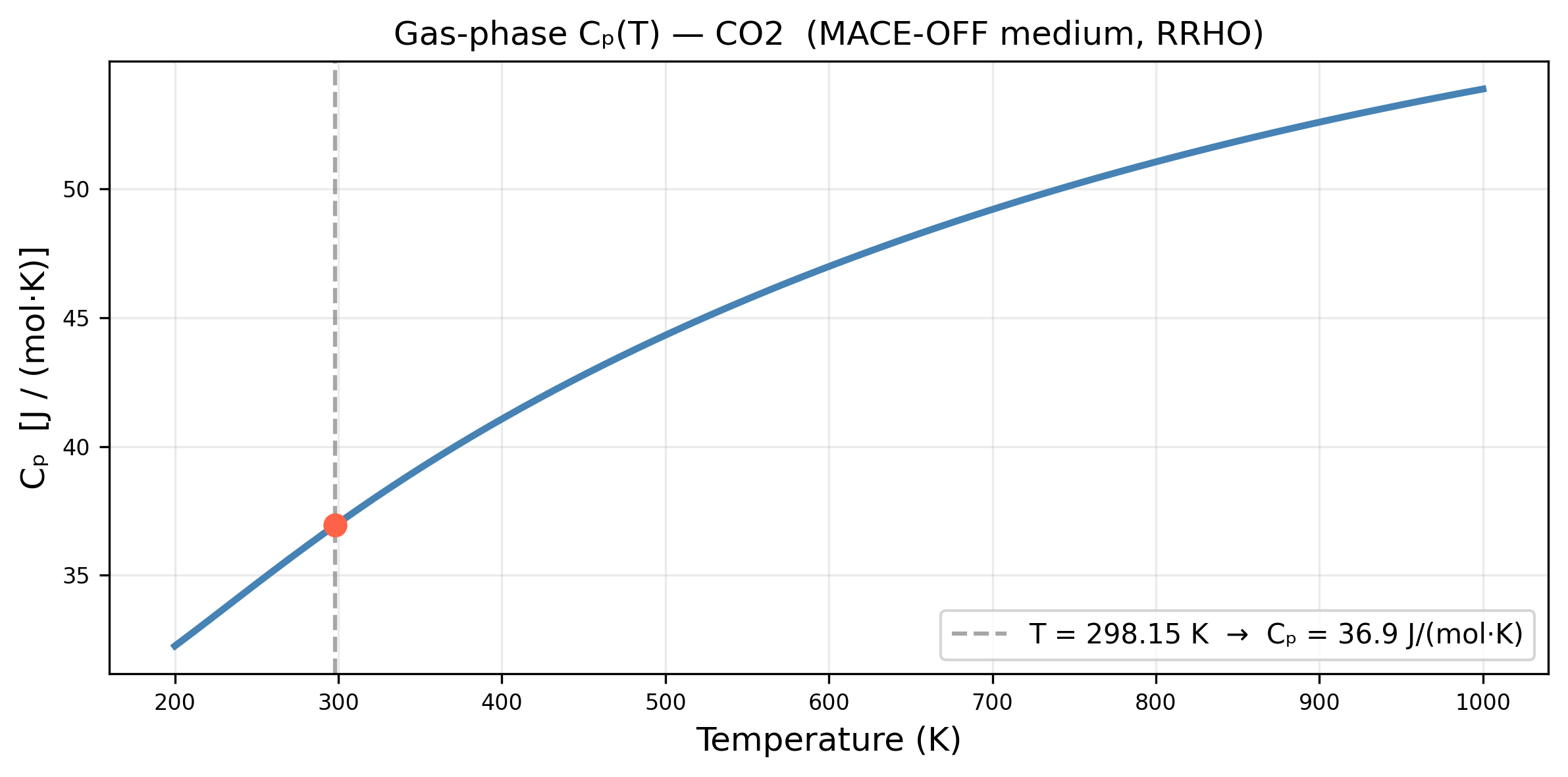
Cell 9 Purpose: Plots the heat capacity as a function of temperature.
# Cell 10: Error between MACE-OFF and NIST (CO2)

# Compute Cp at multiple temperatures
temps_limits_CO2 = [298, 300, 400, 500, 600, 700, 800, 900, 1000, 1100, 1200]
Cp_vals_limits_CO2 = [get_Cp_JmolK(T) for T in temps_limits_CO2]
NIST_Cp_vals_CO2 = [37.12, 37.22, 41.34, 44.61, 47.32, 49.57, 51.44, 53.00, 54.30, 55.40, 56.35]


Cp_vals_limits_CO2 = np.array(Cp_vals_limits_CO2)

data_CO2 = {
    "Temperature in [K]": temps_limits_CO2,
    "Cp [J/mol*K]": Cp_vals_limits_CO2,
    "Percent Error in [%]": np.abs((Cp_vals_limits_CO2 - NIST_Cp_vals_CO2)/NIST_Cp_vals_CO2) * 100,
}

pd.set_option("display.width", 1000)
df = pd.DataFrame(data_CO2)

display(df)

# Comparing Extremely High Temperature Values

# Compute Cp at multiple temperatures
temps_limits_ext_CO2 = [3000, 4000, 5000, 6000]
Cp_vals_limits_ext_CO2 = [get_Cp_JmolK(T) for T in temps_limits_ext_CO2]
NIST_Cp_vals_ext_CO2 = [62.23, 63.25, 64.06, 64.98]


Cp_vals_limits_ext_CO2 = np.array(Cp_vals_limits_ext_CO2)

data_1_CO2 = {
    "Temperature in [K]": temps_limits_ext_CO2,
    "Cp [J/mol*K]": Cp_vals_limits_ext_CO2,
    "Percent Error in [%]": np.abs((Cp_vals_limits_ext_CO2 - NIST_Cp_vals_ext_CO2)/NIST_Cp_vals_ext_CO2) * 100,
}

pd.set_option("display.width", 1000)
df_1 = pd.DataFrame(data_1_CO2)

print("")
display(df_1)
Expected output
	Temperature in [K]	Cp [J/mol*K]	Percent Error in [%]
0	298	36.938209	0.489740
1	300	37.028206	0.515298
2	400	41.068667	0.656344
3	500	44.321863	0.645902
4	600	46.988889	0.699728
5	700	49.203705	0.738944
6	800	51.050402	0.757383
7	900	52.591041	0.771621
8	1000	53.877118	0.778788
9	1100	54.952677	0.807443
10	1200	55.855037	0.878373


Temperature in [K]	Cp [J/mol*K]	Percent Error in [%]
0	3000	61.058247	1.882940
1	4000	61.611573	2.590399
2	5000	61.875708	3.409760
3	6000	62.021393	4.553104
Cell 10 Purpose: Evaluates the difference between MACE-OFF values and NIST values for carbon dioxide.
# Cell 11: This will compute the same information for a different gas (Carbon Monoxide) - Remember to change SMILES, symmetry number, and spin number when changing gases

# You can also change reference Temp (TEMPERATURE_K) to see Cp at different temperatures

SMILES = "[C-]#[O+]"  # Had to play with the SMILES here, C#O did not work (keep this in mind if trying another gas)

TEMPERATURE_K  = 298.15

print("Validating molecule...")
rdkit_mol, formula, mol_weight = validate_smiles(SMILES)

atoms = smiles_to_ase(SMILES)
print(f"3D structure generated: {len(atoms)} atoms")
print(f"Symbols: {atoms.get_chemical_symbols()}")

atoms.calc = calc
print("Optimising geometry with MACE-OFF...")
opt = LBFGS(atoms, logfile=None)
opt.run(fmax=FMAX)

E0 = atoms.get_potential_energy()   # eV
print(f"Optimisation complete.")
print(f"  Energy        : {E0:.6f} eV")
print(f"  Max force     : {np.max(np.linalg.norm(atoms.get_forces(), axis=1)):.4f} eV/Å")


shutil.rmtree("vib_cache", ignore_errors=True)

vib_dir = Path("vib_cache")
vib_dir.mkdir(exist_ok=True)

print(f"Running vibrational analysis ({3 * len(atoms)} force evaluations)...")
vib = Vibrations(atoms, name=str(vib_dir / "vib"), delta=0.01)
vib.run()

# Get all energies
vib_energies = vib.get_energies()

# Filter out imaginary and near-zero frequencies
real_vib_energies = vib_energies[vib_energies.real > 0.01]

# Check for too many imaginary modes
n_imaginary = np.sum(vib_energies.real < 0)
if n_imaginary > 2:
    print(f"⚠️  Warning: {n_imaginary} imaginary frequencies detected.")
    print("    Consider tightening FMAX for more reliable results.")
else:
    print(f"✓  {n_imaginary} imaginary mode(s) filtered — looks clean.")

print(f"\nTotal modes      : {len(vib_energies)}")
print(f"Imaginary/zero   : {len(vib_energies) - len(real_vib_energies)}")
print(f"Real modes kept  : {len(real_vib_energies)}")

# Print frequencies manually in cm⁻¹
print("\nVibrational frequencies (real modes):")
freqs_cm = real_vib_energies.real * 8065.54   # eV → cm⁻¹
for i, f in enumerate(freqs_cm):
    print(f"  Mode {i+1:>3d}: {f:>10.2f} cm⁻¹")


thermo = IdealGasThermo(
    vib_energies=real_vib_energies,
    potentialenergy=E0,
    atoms=atoms,
    geometry='linear',  # Change to match molecule (Linear or nonlinear)
    symmetrynumber=1,   # Change to match molecule (how many times you can turn the molecule and have symmetry)
    spin=1,             # Change to match molecule (0.5 times number of unpaired electrons)
)

Cp_ref = get_Cp_JmolK(TEMPERATURE_K)

print(f"\n{'='*45}")
print(f"  GAS HEAT CAPACITY — {formula}")
print(f"  T = {TEMPERATURE_K} K")
print(f"{'='*45}")
print(f"  Cₚ = {Cp_ref:>8.2f}  J/(mol·K)")
print(f"{'='*45}")

temps = np.linspace(200, 1000, 80)
Cp_vals = [get_Cp_JmolK(T) for T in temps]

fig, ax = plt.subplots(figsize=(8, 4))
ax.plot(temps, Cp_vals, color="steelblue", lw=2.5)
ax.axvline(TEMPERATURE_K, color="gray", ls="--", alpha=0.7,
           label=f"T = {TEMPERATURE_K} K  →  Cₚ = {Cp_ref:.1f} J/(mol·K)")
ax.scatter([TEMPERATURE_K], [Cp_ref], color="tomato", zorder=5, s=60)
ax.set_xlabel("Temperature (K)", fontsize=12)
ax.set_ylabel("Cₚ  [J / (mol·K)]", fontsize=12)
ax.set_title(f"Gas-phase Cₚ(T) — {formula}  (MACE-OFF {MODEL_SIZE}, RRHO)", fontsize=12)
ax.legend(fontsize=10)
ax.grid(True, alpha=0.25)
plt.tight_layout()
plt.show()
Expected output
Validating molecule...
  SMILES   : [C-]#[O+]
  Formula  : CO
  Mol. wt  : 28.01 g/mol
  Elements : {'O', 'C'}
  MACE-OFF compatible: ✓
3D structure generated: 2 atoms
Symbols: ['C', 'O']
Optimising geometry with MACE-OFF...
Optimisation complete.
  Energy        : -3083.920346 eV
  Max force     : 0.0078 eV/Å
Running vibrational analysis (6 force evaluations)...
✓  0 imaginary mode(s) filtered — looks clean.

Total modes      : 6
Imaginary/zero   : 5
Real modes kept  : 1

Vibrational frequencies (real modes):
  Mode   1:    2074.55 cm⁻¹

=============================================
  GAS HEAT CAPACITY — CO
  T = 298.15 K
=============================================
  Cₚ =    29.14  J/(mol·K)
=============================================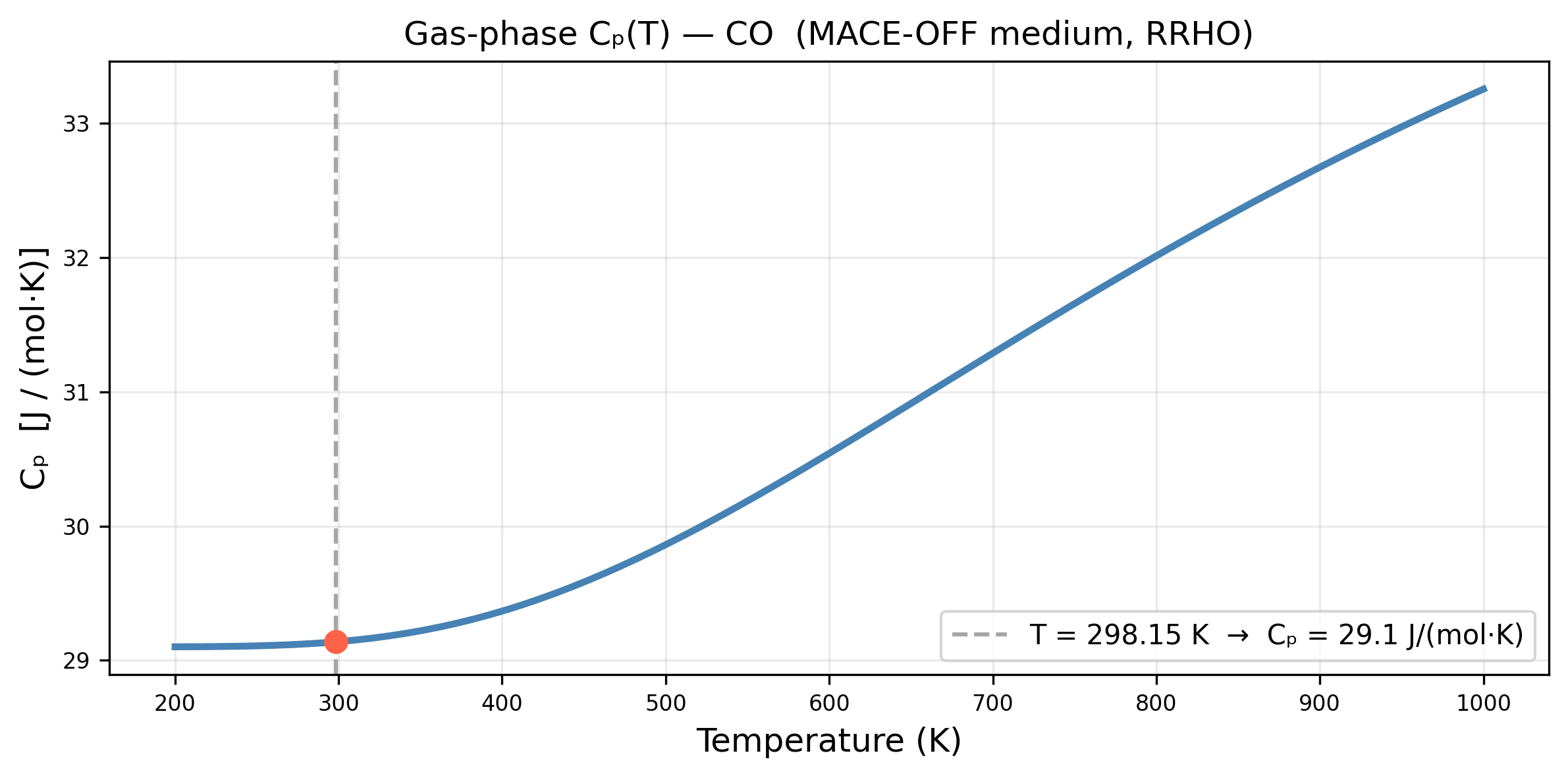
Cell 11 Purpose: Computes the same information from the previous cells except this time for carbon monoxide.
Carbon Monoxide
SMILES: [C-]#[O+]
Chemical Formula: CO
Click the power icon and then run the cell below to view an interactive model of a Carbon Monoxide Molecule
import micropip
await micropip.install("py3Dmol")

from pyodide.http import pyfetch
import py3Dmol


response = await pyfetch("https://raw.githubusercontent.com/cacherowan/CACHE-Rowan/main/Reference_Files/Molecules_To_View/Carbon_Monoxide(CO).xyz")
xyz = await response.string()

view = py3Dmol.view(width=800, height=400)
view.addModel(xyz, "xyz")
view.setStyle({"stick": {}, "sphere": {"scale": 0.3}})
view.zoomTo()
view.zoom(2)
view.show()
# Cell 12: Error between MACE-OFF and NIST (CO)
# Compute Cp at multiple temperatures
temps_limits_CO = [298, 300, 400, 500, 600, 700, 800, 900, 1000, 1100, 1200, 1300]
Cp_vals_limits_CO = [get_Cp_JmolK(T) for T in temps_limits_CO]
NIST_Cp_vals_CO = [29.15, 29.15, 29.30, 29.82, 30.47, 31.17, 31.88, 32.55, 33.18, 33.73, 34.20, 34.55]
Cp_vals_limits_CO = np.array(Cp_vals_limits_CO)
data_CO = {
"Temperature in [K]": temps_limits_CO,
"Cp [J/mol*K]": Cp_vals_limits_CO,
"Percent Error in [%]": np.abs((Cp_vals_limits_CO - NIST_Cp_vals_CO)/NIST_Cp_vals_CO) * 100,
}
pd.set_option("display.width", 1000)
df = pd.DataFrame(data_CO)
display(df)
# Comparing Extremely High Temperature Values
# Compute Cp at multiple temperatures
temps_limits_ext_CO = [3000, 4000, 5000, 6000]
Cp_vals_limits_ext_CO = [get_Cp_JmolK(T) for T in temps_limits_ext_CO]
NIST_Cp_vals_ext_CO = [37.20, 37.72, 38.07, 38.37]
Cp_vals_limits_ext_CO = np.array(Cp_vals_limits_ext_CO)
data_1_CO = {
"Temperature in [K]": temps_limits_ext_CO,
"Cp [J/mol*K]": Cp_vals_limits_ext_CO,
"Percent Error in [%]": np.abs((Cp_vals_limits_ext_CO - NIST_Cp_vals_ext_CO)/NIST_Cp_vals_ext_CO) * 100,
}
pd.set_option("display.width", 1000)
df_1 = pd.DataFrame(data_1_CO)
print("")
display(df_1)Expected output
	Temperature in [K]	Cp [J/mol*K]	Percent Error in [%]
0	298	29.137868	0.041619
1	300	29.139912	0.034606
2	400	29.366873	0.228236
3	500	29.861576	0.139423
4	600	30.542401	0.237615
5	700	31.288024	0.378646
6	800	32.012644	0.416072
7	900	32.673001	0.377884
8	1000	33.254282	0.223876
9	1100	33.756773	0.079373
10	1200	34.187455	0.036682
11	1300	34.555511	0.015950


Temperature in [K]	Cp [J/mol*K]	Percent Error in [%]
0	3000	36.761837	1.177857
1	4000	37.039759	1.803397
2	5000	37.172479	2.357556
3	6000	37.245688	2.930185
Cell 12 Purpose: Evaluates the difference between MACE-OFF values and NIST values for carbon monoxide.
# Cell 13: This will compute the same information for a different gas (Hydrogen Peroxide) - Remember to change SMILES, symmetry number, and spin number when changing gases

# You can also change reference Temp (TEMPERATURE_K) to see Cp at different temperatures

SMILES = "[H]OO[H]"

TEMPERATURE_K  = 298.15

print("Validating molecule...")
rdkit_mol, formula, mol_weight = validate_smiles(SMILES)

atoms = smiles_to_ase(SMILES)
print(f"3D structure generated: {len(atoms)} atoms")
print(f"Symbols: {atoms.get_chemical_symbols()}")

atoms.calc = calc
print("Optimising geometry with MACE-OFF...")
opt = LBFGS(atoms, logfile=None)
opt.run(fmax=FMAX)

E0 = atoms.get_potential_energy()   # eV
print(f"Optimisation complete.")
print(f"  Energy        : {E0:.6f} eV")
print(f"  Max force     : {np.max(np.linalg.norm(atoms.get_forces(), axis=1)):.4f} eV/Å")


shutil.rmtree("vib_cache", ignore_errors=True)

vib_dir = Path("vib_cache")
vib_dir.mkdir(exist_ok=True)

print(f"Running vibrational analysis ({3 * len(atoms)} force evaluations)...")
vib = Vibrations(atoms, name=str(vib_dir / "vib"), delta=0.01)
vib.run()

# Get all energies
vib_energies = vib.get_energies()

# Filter out imaginary and near-zero frequencies
real_vib_energies = vib_energies[vib_energies.real > 0.01]

# Check for too many imaginary modes
n_imaginary = np.sum(vib_energies.real < 0)
if n_imaginary > 2:
    print(f"⚠️  Warning: {n_imaginary} imaginary frequencies detected.")
    print("    Consider tightening FMAX for more reliable results.")
else:
    print(f"✓  {n_imaginary} imaginary mode(s) filtered — looks clean.")

print(f"\nTotal modes      : {len(vib_energies)}")
print(f"Imaginary/zero   : {len(vib_energies) - len(real_vib_energies)}")
print(f"Real modes kept  : {len(real_vib_energies)}")

# Print frequencies manually in cm⁻¹
print("\nVibrational frequencies (real modes):")
freqs_cm = real_vib_energies.real * 8065.54   # eV → cm⁻¹
for i, f in enumerate(freqs_cm):
    print(f"  Mode {i+1:>3d}: {f:>10.2f} cm⁻¹")


thermo = IdealGasThermo(
    vib_energies=real_vib_energies,
    potentialenergy=E0,
    atoms=atoms,
    geometry='nonlinear', # Change to match molecule (Linear or nonlinear)
    symmetrynumber=2,     # Change to match molecule (how many times you can turn the molecule and have symmetry)
    spin=0,               # Change to match molecule (0.5 times number of unpaired electrons)
)

Cp_ref = get_Cp_JmolK(TEMPERATURE_K)

print(f"\n{'='*45}")
print(f"  GAS HEAT CAPACITY — {formula}")
print(f"  T = {TEMPERATURE_K} K")
print(f"{'='*45}")
print(f"  Cₚ = {Cp_ref:>8.2f}  J/(mol·K)")
print(f"{'='*45}")

temps = np.linspace(200, 1000, 80)
Cp_vals = [get_Cp_JmolK(T) for T in temps]

fig, ax = plt.subplots(figsize=(8, 4))
ax.plot(temps, Cp_vals, color="steelblue", lw=2.5)
ax.axvline(TEMPERATURE_K, color="gray", ls="--", alpha=0.7,
           label=f"T = {TEMPERATURE_K} K  →  Cₚ = {Cp_ref:.1f} J/(mol·K)")
ax.scatter([TEMPERATURE_K], [Cp_ref], color="tomato", zorder=5, s=60)
ax.set_xlabel("Temperature (K)", fontsize=12)
ax.set_ylabel("Cₚ  [J / (mol·K)]", fontsize=12)
ax.set_title(f"Gas-phase Cₚ(T) — {formula}  (MACE-OFF {MODEL_SIZE}, RRHO)", fontsize=12)
ax.legend(fontsize=10)
ax.grid(True, alpha=0.25)
plt.tight_layout()
plt.show()
Expected output
Validating molecule...
  SMILES   : [H]OO[H]
  Formula  : H2O2
  Mol. wt  : 34.01 g/mol
  Elements : {'O', 'H'}
  MACE-OFF compatible: ✓
3D structure generated: 4 atoms
Symbols: ['O', 'O', 'H', 'H']
Optimising geometry with MACE-OFF...
Optimisation complete.
  Energy        : -4126.617787 eV
  Max force     : 0.0024 eV/Å
Running vibrational analysis (12 force evaluations)...
✓  0 imaginary mode(s) filtered — looks clean.

Total modes      : 12
Imaginary/zero   : 6
Real modes kept  : 6

Vibrational frequencies (real modes):
  Mode   1:     346.89 cm⁻¹
  Mode   2:    1014.10 cm⁻¹
  Mode   3:    1413.11 cm⁻¹
  Mode   4:    1575.46 cm⁻¹
  Mode   5:    3818.13 cm⁻¹
  Mode   6:    3843.96 cm⁻¹

=============================================
  GAS HEAT CAPACITY — H2O2
  T = 298.15 K
=============================================
  Cₚ =    42.05  J/(mol·K)
=============================================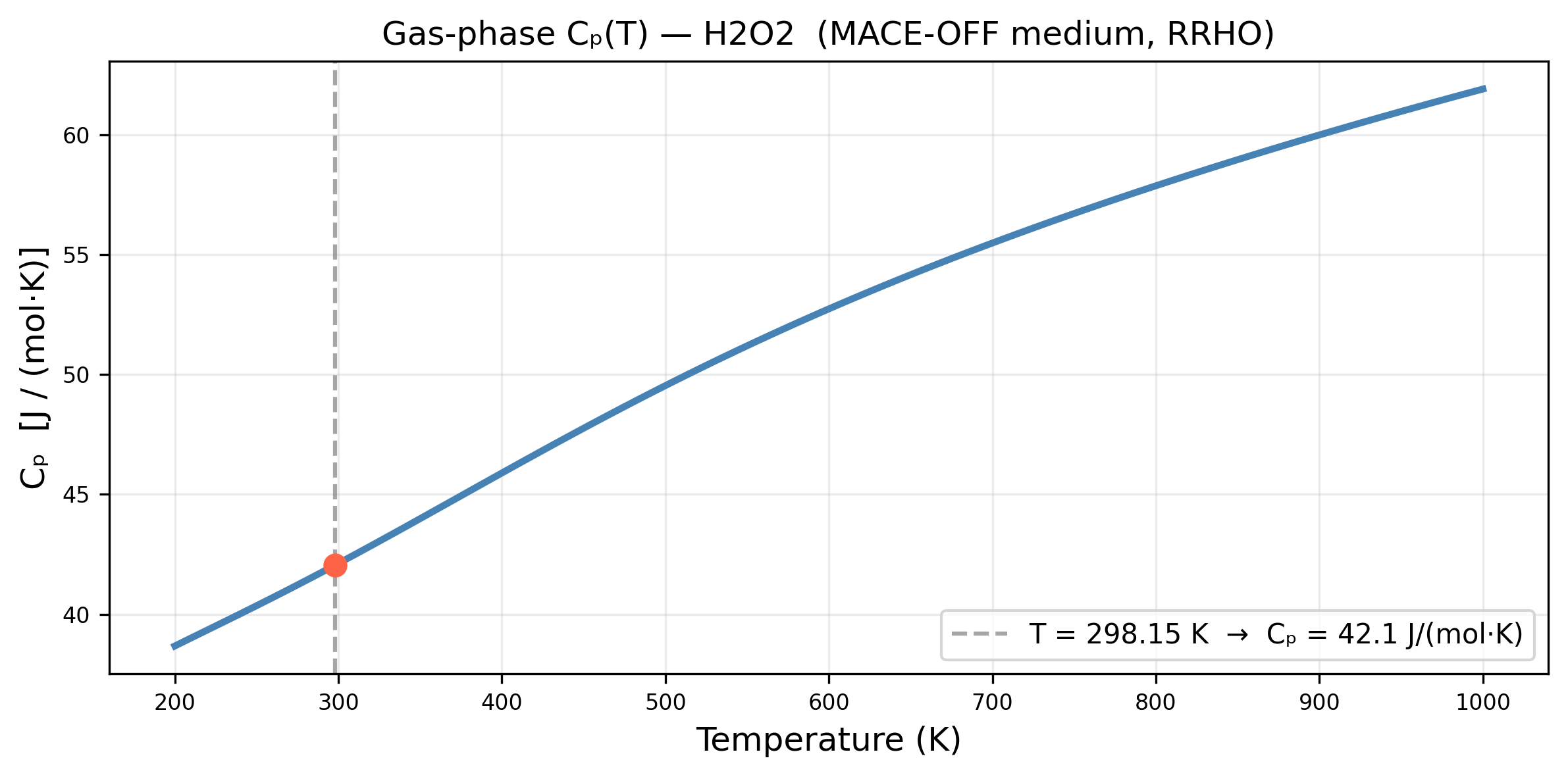
Cell 13 Purpose: Computes the same information from the previous cells except this time for hydrogen peroxide.
Hydrogen Peroxide
SMILES: [H]OO[H]
Chemical Formula: H2O2
Click the power icon and then run the cell below to view an interactive model of a Hydrogen Peroxide Molecule
import micropip
await micropip.install("py3Dmol")

from pyodide.http import pyfetch
import py3Dmol


response = await pyfetch("https://raw.githubusercontent.com/cacherowan/CACHE-Rowan/main/Reference_Files/Molecules_To_View/Hydrogen_Peroxide(H2O2).xyz")
xyz = await response.string()

view = py3Dmol.view(width=800, height=400)
view.addModel(xyz, "xyz")
view.setStyle({"stick": {}, "sphere": {"scale": 0.3}})
view.zoomTo()
view.zoom(2)
view.show()
# Cell 14: Error between MACE-OFF and NIST (H2O2)
# Compute Cp at multiple temperatures
temps_limits_H2O2 = [298, 300, 400, 500, 600, 700, 800, 900, 1000, 1100, 1200, 1300, 1400, 1500]
Cp_vals_limits_H2O2 = [get_Cp_JmolK(T) for T in temps_limits_H2O2]
NIST_Cp_vals_H2O2 = [43.07, 43.20, 48.65, 52.51, 55.50, 57.92, 59.90, 61.55, 62.95, 64.17, 65.27, 66.30, 67.33, 68.42]
Cp_vals_limits_H2O2 = np.array(Cp_vals_limits_H2O2)
data_H2O2 = {
"Temperature in [K]": temps_limits_H2O2,
"Cp [J/mol*K]": Cp_vals_limits_H2O2,
"Percent Error in [%]": np.abs((Cp_vals_limits_H2O2 - NIST_Cp_vals_H2O2)/NIST_Cp_vals_H2O2) * 100,
}
pd.set_option("display.width", 1000)
df = pd.DataFrame(data_H2O2)
display(df)Expected output
Temperature in [K]	Cp [J/mol*K]	Percent Error in [%]
0	298	42.047975	2.372940
1	300	42.120797	2.498155
2	400	45.893051	5.666904
3	500	49.538508	5.658906
4	600	52.740797	4.971536
5	700	55.487803	4.199235
6	800	57.875608	3.379619
7	900	59.996516	2.523939
8	1000	61.911483	1.649748
9	1100	63.655332	0.802038
10	1200	65.247597	0.034324
11	1300	66.700623	0.604259
12	1400	68.024088	1.030875
13	1500	69.227024	1.179515
Cell 14 Purpose: Evaluates the difference between MACE-OFF values and NIST values for hydrogen peroxide.
# Cell 15: This will compute the same information for a different gas (Methane) - Remember to change SMILES, symmetry number, and spin number when changing gases

# You can also change reference Temp (TEMPERATURE_K) to see Cp at different temperatures

SMILES = "C"

TEMPERATURE_K  = 298.15

print("Validating molecule...")
rdkit_mol, formula, mol_weight = validate_smiles(SMILES)

atoms = smiles_to_ase(SMILES)
print(f"3D structure generated: {len(atoms)} atoms")
print(f"Symbols: {atoms.get_chemical_symbols()}")

atoms.calc = calc
print("Optimising geometry with MACE-OFF...")
opt = LBFGS(atoms, logfile=None)
opt.run(fmax=FMAX)

E0 = atoms.get_potential_energy()   # eV
print(f"Optimisation complete.")
print(f"  Energy        : {E0:.6f} eV")
print(f"  Max force     : {np.max(np.linalg.norm(atoms.get_forces(), axis=1)):.4f} eV/Å")

shutil.rmtree("vib_cache", ignore_errors=True)

vib_dir = Path("vib_cache")
vib_dir.mkdir(exist_ok=True)

print(f"Running vibrational analysis ({3 * len(atoms)} force evaluations)...")
vib = Vibrations(atoms, name=str(vib_dir / "vib"), delta=0.01)
vib.run()

# Get all energies
vib_energies = vib.get_energies()

# Filter out imaginary and near-zero frequencies
real_vib_energies = vib_energies[vib_energies.real > 0.01]

# Check for too many imaginary modes
n_imaginary = np.sum(vib_energies.real < 0)
if n_imaginary > 2:
    print(f"⚠️  Warning: {n_imaginary} imaginary frequencies detected.")
    print("    Consider tightening FMAX for more reliable results.")
else:
    print(f"✓  {n_imaginary} imaginary mode(s) filtered — looks clean.")

print(f"\nTotal modes      : {len(vib_energies)}")
print(f"Imaginary/zero   : {len(vib_energies) - len(real_vib_energies)}")
print(f"Real modes kept  : {len(real_vib_energies)}")

# Print frequencies manually in cm⁻¹
print("\nVibrational frequencies (real modes):")
freqs_cm = real_vib_energies.real * 8065.54   # eV → cm⁻¹
for i, f in enumerate(freqs_cm):
    print(f"  Mode {i+1:>3d}: {f:>10.2f} cm⁻¹")


thermo = IdealGasThermo(
    vib_energies=real_vib_energies,
    potentialenergy=E0,
    atoms=atoms,
    geometry='nonlinear', # Change to match molecule (Linear or nonlinear)
    symmetrynumber=12,     # Change to match molecule (how many times you can turn the molecule and have symmetry)
    spin=0,               # Change to match molecule (0.5 times number of unpaired electrons)
)

Cp_ref = get_Cp_JmolK(TEMPERATURE_K)

print(f"\n{'='*45}")
print(f"  GAS HEAT CAPACITY — {formula}")
print(f"  T = {TEMPERATURE_K} K")
print(f"{'='*45}")
print(f"  Cₚ = {Cp_ref:>8.2f}  J/(mol·K)")
print(f"{'='*45}")

temps = np.linspace(200, 1000, 80)
Cp_vals = [get_Cp_JmolK(T) for T in temps]

fig, ax = plt.subplots(figsize=(8, 4))
ax.plot(temps, Cp_vals, color="steelblue", lw=2.5)
ax.axvline(TEMPERATURE_K, color="gray", ls="--", alpha=0.7,
           label=f"T = {TEMPERATURE_K} K  →  Cₚ = {Cp_ref:.1f} J/(mol·K)")
ax.scatter([TEMPERATURE_K], [Cp_ref], color="tomato", zorder=5, s=60)
ax.set_xlabel("Temperature (K)", fontsize=12)
ax.set_ylabel("Cₚ  [J / (mol·K)]", fontsize=12)
ax.set_title(f"Gas-phase Cₚ(T) — {formula}  (MACE-OFF {MODEL_SIZE}, RRHO)", fontsize=12)
ax.legend(fontsize=10)
ax.grid(True, alpha=0.25)
plt.tight_layout()
plt.show()
Expected output
Validating molecule...
  SMILES   : C
  Formula  : CH4
  Mol. wt  : 16.04 g/mol
  Elements : {'C', 'H'}
  MACE-OFF compatible: ✓
3D structure generated: 5 atoms
Symbols: ['C', 'H', 'H', 'H', 'H']
Optimising geometry with MACE-OFF...
Optimisation complete.
  Energy        : -1103.060054 eV
  Max force     : 0.0016 eV/Å
Running vibrational analysis (15 force evaluations)...
✓  0 imaginary mode(s) filtered — looks clean.

Total modes      : 15
Imaginary/zero   : 6
Real modes kept  : 9

Vibrational frequencies (real modes):
  Mode   1:    1333.47 cm⁻¹
  Mode   2:    1333.55 cm⁻¹
  Mode   3:    1333.71 cm⁻¹
  Mode   4:    1544.11 cm⁻¹
  Mode   5:    1544.29 cm⁻¹
  Mode   6:    3056.75 cm⁻¹
  Mode   7:    3162.55 cm⁻¹
  Mode   8:    3162.71 cm⁻¹
  Mode   9:    3162.93 cm⁻¹

=============================================
  GAS HEAT CAPACITY — CH4
  T = 298.15 K
=============================================
  Cₚ =    35.46  J/(mol·K)
=============================================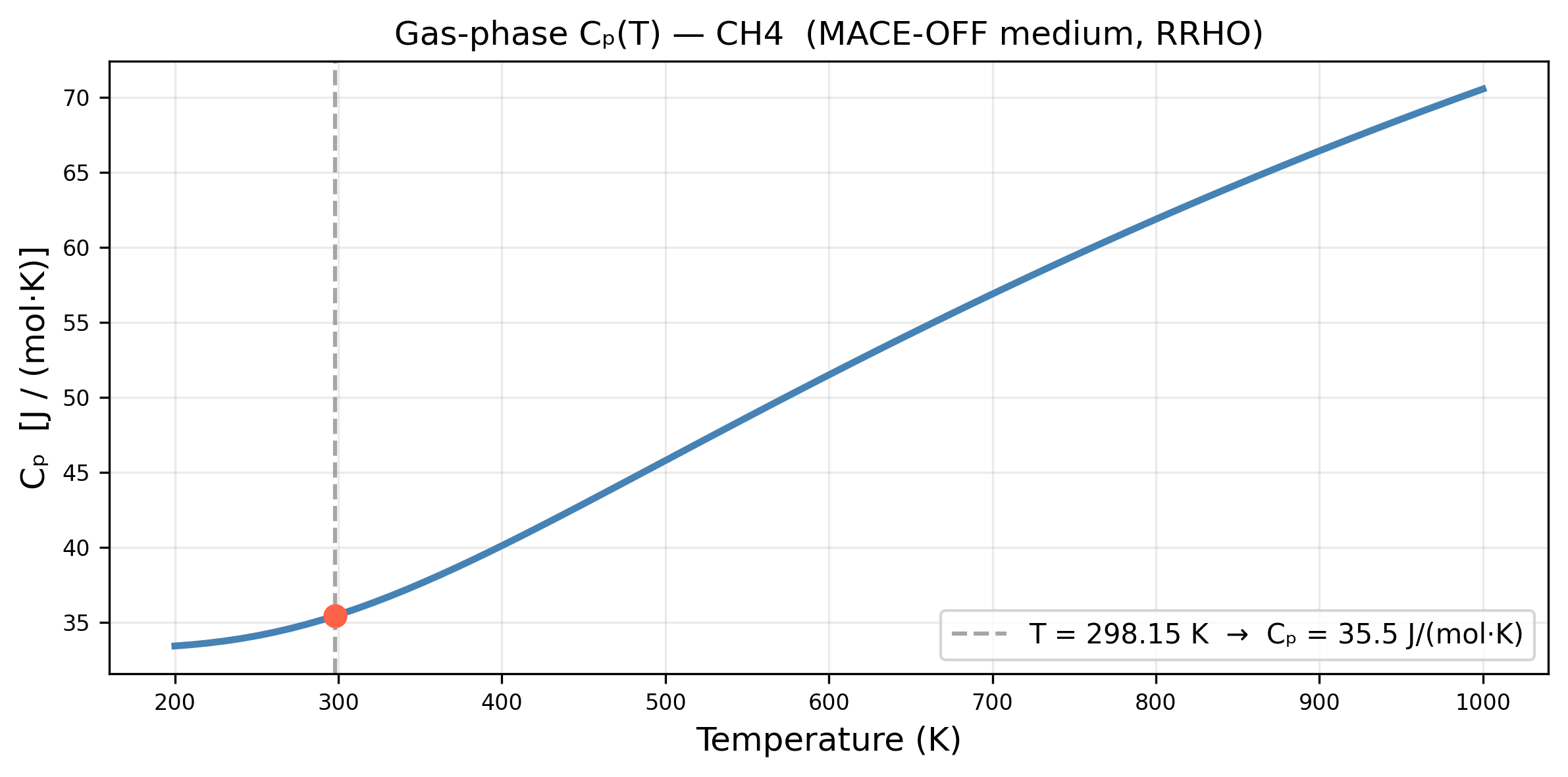
Cell 15 Purpose: Computes the same information from the previous cells except this time for methane.
Methane
SMILES: C
Chemical Formula: CH4
Click the power icon and then run the cell below to view an interactive model of a Methane Molecule
import micropip
await micropip.install("py3Dmol")

from pyodide.http import pyfetch
import py3Dmol


response = await pyfetch("https://raw.githubusercontent.com/cacherowan/CACHE-Rowan/main/Reference_Files/Molecules_To_View/Methane(CH4).xyz")
xyz = await response.string()

view = py3Dmol.view(width=800, height=400)
view.addModel(xyz, "xyz")
view.setStyle({"stick": {}, "sphere": {"scale": 0.3}})
view.zoomTo()
view.zoom(2)
view.show()
# Cell 16: Error between MACE-OFF and NIST (CH4)
# Compute Cp at multiple temperatures
temps_limits_CH4 = [298, 300, 400, 500, 600, 700, 800, 900, 1000, 1100, 1200, 1300]
Cp_vals_limits_CH4 = [get_Cp_JmolK(T) for T in temps_limits_CH4]
NIST_Cp_vals_CH4 = [35.69, 35.76, 40.63, 46.63, 52.74, 58.60, 64.08, 69.14, 73.75, 77.92, 81.68, 85.07]
Cp_vals_limits_CH4 = np.array(Cp_vals_limits_CH4)
data_CH4 = {
"Temperature in [K]": temps_limits_CH4,
"Cp [J/mol*K]": Cp_vals_limits_CH4,
"Percent Error in [%]": np.abs((Cp_vals_limits_CH4 - NIST_Cp_vals_CH4)/NIST_Cp_vals_CH4) * 100,
}
pd.set_option("display.width", 1000)
df = pd.DataFrame(data_CH4)
display(df)
# Comparing Extremely High Temperature Values
# Compute Cp at multiple temperatures
temps_limits_ext_CH4 = [2000, 2500, 3000]
Cp_vals_limits_ext_CH4 = [get_Cp_JmolK(T) for T in temps_limits_ext_CH4]
NIST_Cp_vals_ext_CH4 = [101.24, 108.23, 113.55]
Cp_vals_limits_ext_CH4 = np.array(Cp_vals_limits_ext_CH4)
data_1_CH4 = {
"Temperature in [K]": temps_limits_ext_CH4,
"Cp [J/mol*K]": Cp_vals_limits_ext_CH4,
"Percent Error in [%]": np.abs((Cp_vals_limits_ext_CH4 - NIST_Cp_vals_ext_CH4)/NIST_Cp_vals_ext_CH4) * 100,
}
pd.set_option("display.width", 1000)
df_1 = pd.DataFrame(data_1_CO)
print("")
display(df_1)Expected output
Temperature in [K]	Cp [J/mol*K]	Percent Error in [%]
0	298	35.453303	0.663202
1	300	35.523286	0.661953
2	400	40.130441	1.229533
3	500	45.805146	1.768934
4	600	51.516004	2.320812
5	700	56.908704	2.886171
6	800	61.893504	3.412135
7	900	66.448430	3.892927
8	1000	70.571158	4.310295
9	1100	74.272452	4.681145
10	1200	77.574359	5.026495
11	1300	80.506991	5.363829


Temperature in [K]	Cp [J/mol*K]	Percent Error in [%]
0	3000	36.761837	1.177857
1	4000	37.039759	1.803397
2	5000	37.172479	2.357556
3	6000	37.245688	2.930185
Cell 16 Purpose: Evaluates the difference between MACE-OFF values and NIST values for methane.
Discusion / Analysis
In this code, carbon dioxide, carbon monoxide, hydrogen peroxide, and methane were all simulated to estimate their heat capacities at different temperatures using ASE and MACE-OFF. We then compared the error in MACE-OFF and NIST to see how close they were. From the results you can see the error percentage was extremely low. When looking into how NIST calculated their Cp at certain temperatures, it turns out, they also use a Rigid-Rotor Harmonic-Oscillator assumption for their values, so the error comparison ends up being between how well each calculated frequencies of the molecules. Also keep in mind generally as temperature increases, different vibrational mode can occur, so the error could be higher as temperature increases, which is an interesting lens to look at the error again through.